Pivot tables in Python

A Pivot Table is a related operation which is commonly seen in spreadsheets and other programs which operate on tabular data. The Pivot Table takes simple column-wise data as input, and groups the entries into a two-dimensional table which provides a multi-dimensional summarization of the data. The difference between Pivot Tables and GroupBy can sometimes cause confusion; it helps me to think of pivot tables as essentially a multi-dimensional version of GroupBy aggregation. That is, you split-apply-combine, but both the split and the combine happen across not a one-dimensional index, but across a two-dimensional grid.

Motivating Pivot Tables

For the examples in this section, we’ll use the database of passengers on the Titanic, available through the seaborn library:

import numpy as np
import pandas as pd
import seaborn as sns
titanic = sns.load_dataset('titanic')

titanic.head()

This contains a wealth of information on each passenger of that ill-fated voyage, including their gender, age, class, fare paid, and much more.

Pivot Tables By Hand

To start learning more about this data, we might want to like to group it by gender, survival, or some combination thereof. If you have read the previous section, you might be tempted to apply a GroupBy operation to this data. For example, let’s look at survival rate by gender:

titanic.groupby('sex')[['survived']].mean()

This immediately gives us some insight: overall three of every four females on board survived, while only one in five males survived!

This is an interesting insight, but we might like to go one step deeper and look at survival by both sex and, say, class. Using the vocabulary of GroupBy, we might proceed something like this: We group by class and gender, select survival, apply a mean aggregate, combine the resulting groups, and then unstack the hierarchical index to reveal the hidden multidimensionality. In code:

titanic.groupby(['sex', 'class'])['survived'].aggregate('mean').unstack()

This gives us a better idea of how both gender and class affected survival, but the code is starting to look a bit garbled. While each step of this pipeline makes sense in light of the tools we’ve previously discussed, the long string of code is not particularly easy to read or use. This type of operation is common enough that Pandas includes a convenience routine, pivot_table, which succinctly handles this type of multi-dimensional aggregation.

Pivot Table Syntax

Here is the equivalent to the above operation using the pivot_table method of dataframes:

titanic.pivot_table('survived', index='sex', columns='class')

This is eminently more readable than the equivalent GroupBy operation, and produces the same result. As you might expect of an early 20th century transatlantic cruise, the survival gradient favors both women and higher classes. First-class women survived with near certainty (hi Kate!), while only one in ten third-class men survived (sorry Leo!).

Multi-level Pivot Tables

Just as in the GroupBy, the grouping in pivot tables can be specified with multiple levels, and via a number of options. For example, we might be interested in looking at age as a third dimension. We’ll bin the age using the pd.cut function:

age = pd.cut(titanic['age'], [0, 18, 80])
titanic.pivot_table('survived', ['sex', age], 'class')

we can do the same game with the columns; let’s add info on the fare paid using pd.qcut to automatically compute quantiles:

fare = pd.qcut(titanic['fare'], 2)
titanic.pivot_table('survived', ['sex', age], [fare, 'class'])

The result is a four-dimensional aggregation, shown in a grid which demonstrates the relationship between the values.

Additional Pivot Table Options

The full call signature of the pivot_table method of DataFrames is as follows:

DataFrame.pivot_table(values=None, index=None, columns=None, aggfunc='mean',
                      fill_value=None, margins=False, dropna=True)

Above we’ve seen examples of the first three arguments; here we’ll take a quick look at the remaining arguments. Two of the options, fill_value and dropna, have to do with missing data and are fairly straightforward; we will not show examples of them here.

The aggfunc keyword controls what type of aggregation is applied, which is a mean by default. As in the GroupBy, the aggregation specification can be a string representing one of several common choices (e.g. 'sum', 'mean', 'count', 'min', 'max', etc.) or a function which implements an aggregation (e.g. np.sum(), min(), sum(), etc.). Additionally, it can be specified as dictionary mapping a column to any of the above desired options:

titanic.pivot_table(index='sex', columns='class',
								aggfunc={'survived':sum, 'fare':'mean'})

Notice also here that we’ve omitted the values keyword; when specifying a mapping for aggfunc, this is determined automatically.

At times it’s useful to compute totals along each grouping. This can be done via the margins keyword:

titanic.pivot_table('survived', index='sex', columns='class', margins=True)

Here this automatically gives us information about the class-agnostic survival rate by gender, the gender-agnostic survival rate by class, and the overall survival rate of 38%.

Example: Birthrate Data

As a more interesting example, let’s take a look at the freely-available data on births in the USA, provided by the Centers for Disease Control (CDC). This data can be found at https://raw.githubusercontent.com/jakevdp/data-CDCbirths/master/births.csv This dataset has been analyzed rather extensively by Andrew Gelman and his group; see for example this blog post.

# shell command to download the data:
!curl -O https://raw.githubusercontent.com/jakevdp/data-CDCbirths/master/births.csv

births = pd.read_csv('births.csv')

Taking a look at the data, we see that it’s relatively simple: it contains the number of births grouped by date and gender:

births.head()

We can start to understand this data a bit more by using a pivot table. Let’s add a decade column, and take a look at male and female births as a function of decade:

births['decade'] = 10 * (births['year'] // 10)
births.pivot_table('births', index='decade', columns='gender', aggfunc='sum')

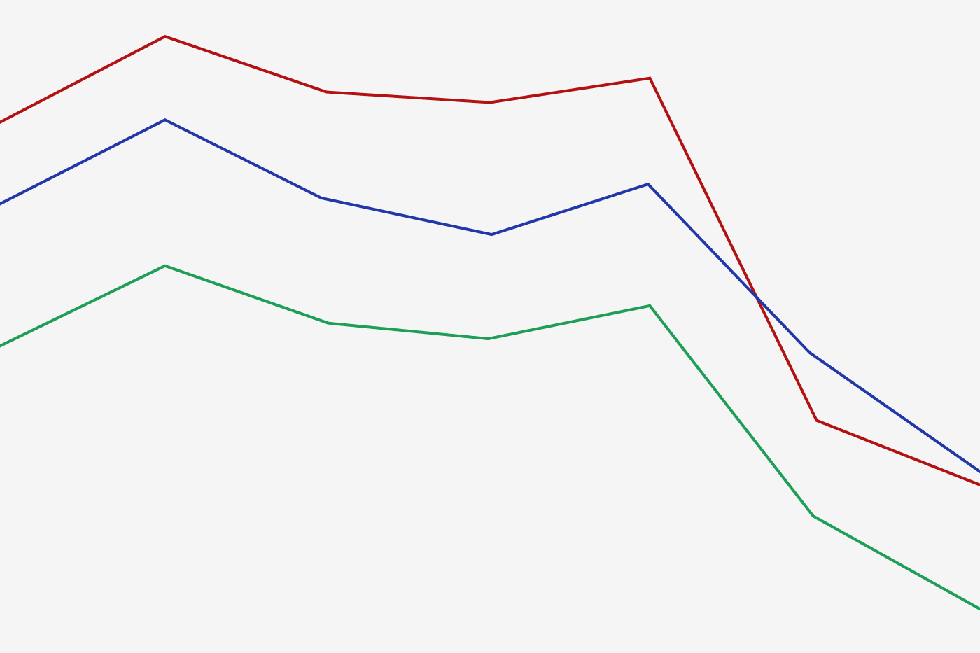
We immediately see that male births outnumber female births in every decade. To see this trend a bit more clearly, we can use Pandas’ built-in plotting tools to visualize the total number of births by year (see Chapter X.X for a discussion of plotting with matplotlib):

%matplotlib inline
import matplotlib.pyplot as plt
sns.set()  # use seaborn styles
births.pivot_table('births', index='year', columns='gender', aggfunc='sum').plot()
plt.ylabel('total births per year');

With a simple pivot table and plot() method, we can immediately see the annual trend in births by gender. By eye, we find that over the past 50 years male births have outnumbered female births by around 5%.

Further Data Exploration

Though this doesn’t necessarily relate to the pivot table, there are a few more interesting features we can pull out of this dataset using the Pandas tools covered up to this point. We must start by cleaning the data a bit, removing outliers caused by mistyped dates (e.g. June 31st) or missing values (e.g. June 99th). One easy way to remove these all at once is to cut outliers; we’ll do this via a robust sigma-clipping operation:

# Some data is mis-reported; e.g. June 31st, etc.
# remove these outliers via robust sigma-clipping
quartiles = np.percentile(births['births'], [25, 50, 75])
mu = quartiles[1]
sig = 0.7413 * (quartiles[2] - quartiles[0])
births = births.query('(births > @mu - 5 * @sig) & (births < @mu + 5 * @sig)')

Next we set the day column to integers; previously it had been a string because some columns in the dataset contained the value 'null':

# set 'day' column to integer; it originally was a string due to nulls
births['day'] = births['day'].astype(int)

Finally, we can combine the day, month, and year to create a Date index (see section X.X). This allows us to quickly compute the weekday corresponding to each row:

# create a datetime index from the year, month, day
births.index = pd.to_datetime(10000 * births.year +
													100 * births.month +
													births.day, format='%Y%m%d')

births['dayofweek'] = births.index.dayofweek

Using this we can plot births by weekday for several decades:

import matplotlib.pyplot as plt
import matplotlib as mpl

births.pivot_table('births', index='dayofweek',
								columns='decade', aggfunc='mean').plot()
plt.gca().set_xticklabels(['Mon', 'Tues', 'Wed', 'Thurs', 'Fri', 'Sat', 'Sun'])
plt.ylabel('mean births by day');

Apparently births are slightly less common on weekends than on weekdays! Note that the 1990s and 2000s are missing because the CDC stopped reports only the month of birth starting in 1989.

Another intersting view is to plot the mean number of births by the day of the year. We can do this by constructing a datetime array for a particular year, making sure to choose a leap year so as to account for February 29th.

# Choose a leap year to display births by date
dates = [pd.datetime(2012, month, day)
		for (month, day) in zip(births['month'], births['day'])]

We can now group by the data by day of year and plot the results. We’ll additionally annotate the plot with the location of several US holidays:

# Plot the results
fig, ax = plt.subplots(figsize=(8, 6))
births.pivot_table('births', dates).plot(ax=ax)

# Label the plot
ax.text('2012-1-1', 3950, "New Year's Day")
ax.text('2012-7-4', 4250, "Independence Day", ha='center')
ax.text('2012-9-4', 4850, "Labor Day", ha='center')
ax.text('2012-10-31', 4600, "Halloween", ha='right')
ax.text('2012-11-25', 4450, "Thanksgiving", ha='center')
ax.text('2012-12-25', 3800, "Christmas", ha='right')
ax.set(title='USA births by day of year (1969-1988)',
	ylabel='average daily births',
	xlim=('2011-12-20','2013-1-10'),
	ylim=(3700, 5400));

# Format the x axis with centered month labels
ax.xaxis.set_major_locator(mpl.dates.MonthLocator())
ax.xaxis.set_minor_locator(mpl.dates.MonthLocator(bymonthday=15))
ax.xaxis.set_major_formatter(plt.NullFormatter())
ax.xaxis.set_minor_formatter(mpl.dates.DateFormatter('%h'));

The lower birthrate on holidays is striking, but is likely the result of selection for scheduled/induced births rather than any deep psychosomatic causes. For more discussion on this trend, see the discussion and links in Andrew Gelman’s blog posts on the subject.

This short example should give you a good idea of how many of the Pandas tools we’ve seen to this point can be put together and used to gain insight from a variety of datasets. We will see some more sophisticated analysis of this data, and other datasets like it, in future sections!